Self Flying Drone
- Yash Aryan

- Jul 27, 2020
- 15 min read
OVERVIEW :
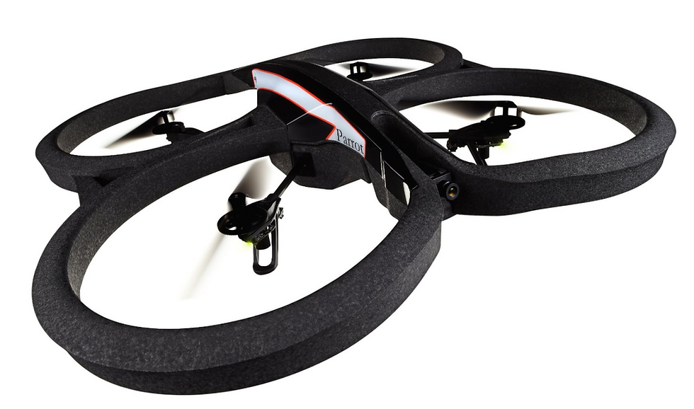
The Quadcopter or Quadrotor Helicopter is becoming an increasingly popular aircraft for both personal and professional use. Its maneuverability lends itself to many applications, from last-mile delivery to cinematography, from acrobatics to search-and-rescue.
The next step in this evolution is to enable Quadcopters to autonomously achieve desired control behaviors such as takeoff and landing. You could design these controls with a classic approach (say, by implementing PID controllers). Or, you can use reinforcement learning to build agents that can learn these behaviors on their own. This is what we are going to do in this project!
Installation Dependencies:
Matplotlib==2.0.0
Numpy==1.14.1
Pandas==0.19.2
Python 2.7
Keras 1.1.0
Tensorflow r0.10
Important Files :
Github Link : https://github.com/yash143/Self-Flying-drone/tree/master
Follow me along with the Jupyter Notebook (Self_flying_drone.ipynb)provided in the link above .
Motivation:
Since my childhood I always have had interest in remote control cars , Robots , Drones and everything that uses AI but I never had enough money to buy them at that time .Although we are still far away from building super-intelligent AI system, the latest development in the computer vision ,Reinforcement learning and deep learning has created an exciting era for me to at least fulfill my little dream now of creating AI systems.
Background:
As we know that recent advancements Q-Learning resulting in Deep Q-Learning has made life simpler in many ways. However, a big limitation of Deep Q-Network is that the outputs/actions are discrete while the action like steering are continuous if you consider the example of a car. An obvious approach to adapt DQN to continuous domains is to simply discretize the action space. However, we encounter the “curse of dimensionality problem. For example, if you discretize the steering wheel from -90 to +90 degrees in 5 degrees each and acceleration from 0km to 300km in 5km each, your output combinations will be 36 steering states times 60 velocity states which equals to 2160 possible combinations. The situation will be worse when you want to build robots to perform something very specialized, such as brain surgery that requires fine control of actions and naive discretization will not able to achieve the required precision to do the operations.I hope this example is convincing enough why DQN is not suitable for all the tasks.
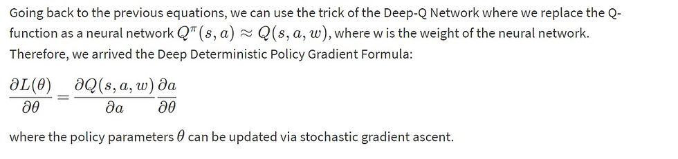
Google Deepmind has devised a new algorithm to tackle the continuous action space problem by combining 3 techniques together 1) Deterministic Policy-Gradient Algorithms 2) Actor-Critic Methods 3) Deep Q-Network called Deep Deterministic Policy Gradients (DDPG)
Simulator(physics) For The Drone (Optional):
File : Drone_physics.py
Those who are interested in the physics behind the working of Quadcopter , lets dive right in.
In simple terms as power flows from the batteries to the rotor motors, the propellers begin to spin, and it's the spin of each prop relative to the others that changes altitude and direction. Rev up the rotors and they'll generate enough lift to overcome the force of gravity, zipping the drone higher and higher.But the Physics behind it is far more complicated than it seems .So I will try to simplify it as much as possible.
First we need to shift the frames as Inertial frames axes are earth fixed and body frame axes are aligned with the drone as shown in the figure below .

we can use the following function/Matrix to shift the frame .
def earth_to_body_frame(ii, jj, kk):

    R = [[Cos(kk)*Cos(jj), Cos(kk)*Sin(jj)*Sin(ii)-Sin(kk)*Cos(ii),
             Cos(kk) * Sin(jj) * Cos(ii) + Sin(kk) * Sin(ii)],
         [Sin(kk)*Cos(jj), Sin(kk)*Sin(jj)*Sin(ii)+Cos(kk)*Cos(ii),
             Sin(kk)*Sin(jj)*Cos(ii)-Cos(kk)*Sin(ii)],
         [-Sin(jj), Cos(jj)*Sin(ii), Cos(jj)*Cos(ii)]]
    return np.array(R)
where ii=phi , jj=theta , kk=psi are Euler angles . Transpose of R gives the Body frame to earth frame converter matrix. So when you multiply a vector in inertial frame [x,y,z] with R you get the representation of that vector with respect to body frame .
In our project the drone consist of 4 rotors .The agent controls drone by setting the revolutions per second on each of its four rotors .Hence our Action Space is of size 4.
Position of drone is defined by (x,y,z) and Euler angles phi , theta and psi ([x,y,z,phi,theta,psi]) at any time step t .Our ultimate goal is to change the position of drone after each time step .
To change the x,y,z components we need to calculate the acceleration of drone because Position[x , y , z] = intial_pos[x,y,z] + velocity[x,y,z] *dt + 0.5 * acceleration[x,y,z]* dt*dt.
We know that linear_acceleration = linear_forces / mass of drone .So linear_forces can be calculated from the function below .
def find_body_velocity():
        body_velocity =
        np.matmul(earth_to_body_frame(*list([x ,y ,z ])),
        velocity[x,y,z])
        return body_velocity
def get_linear_drag():
        (areas = np.array([length * height, width * height, width
        *length]) , #rho=density of air , #C_d=drag coefficient)

        linear_drag = 0.5 * rho * find_body_velocity()**2 *
        areas_of_drone * C_d

        return linear_drag
def get_linear_forces(self, thrusts):
        # Gravity
        gravity_force = mass * gravity * np.array([0, 0, 1])
        # Thrust
        thrust_body_force = np.array([0, 0, sum(thrusts)])
        # Drag
        drag_body_force = -get_linear_drag()
        body_forces = thrust_body_force + drag_body_force

        linear_forces =
        np.matmul(body_to_earth_frame(*list([x,y,z])),
        body_forces)
        linear_forces += gravity_force
        return linear_forces
And now we can finally update values of [x ,y, z] after calculating linear_forces.
Now to update Euler angles phi , theta and psi we similary need angular acceleration.
Angles[phi , theta, psi] = Intial_Angles[phi,theta,psi] + angular_velocity * self.dt + 0.5 * angular_accels*self.angular_accels * self.dt ** 2
angular_accels = moments / moments_of_inertia . So moments can be calculated from the function below.
I_x = 1 / 12. * mass * (height**2 + width**2)
I_y = 1 / 12. * mass * (height**2 + length**2)
I_z = 1 / 12. * mass * (width**2 + length**2)
moments_of_inertia = np.array([I_x, I_y, I_z])  # moments of inertia
def get_moments(thrusts):
thrust_moment = np.array([(thrusts[3] -
thrusts[2])*self.l_to_rotor,(thrusts[1] - thrusts[0]) *
self.l_to_rotor,0])
drag_moment = C_d * 0.5 * rho * angular_v *
np.absolute(angular_v) *areas *dims *dims
moments = thrust_moment - drag_moment # + motor_inertia_moment
return momentsAnd now we can finally update phi , theta and psi .
So our entire state array [ x , y , z , phi , theta , psi ] will be updated after each time step resulting in a new state .
Entire Code of above Simulation is provided in Drone_physics.py
Important:
State Space = [x , y , z , phi , theta ,psi]
Action space = [ v1 , v2 , v3 , v4] (Speeds of 4 rotors)
Policy Network :
First, we are going to define a policy network that implements our AI-driver. This network will take the state of the drone ([x , y , z , phi , theta , psi]) and decide the action (Speed of 4 rotors). It is called Policy-Based Reinforcement Learning because we will directly parametrize the policy
πθ(s,a)=P[a∣s,θ]
here, s is the state , a is the action and θ is the model parameters of the policy network. We can think of policy is the agent’s behaviour, i.e. a function to map from state to action.
Deterministic vs Stochastic Policy :
Please note that there are 2 types of the policies:
Deterministic policy: a=μ(s)
Stochastic policy: π(a∣s)=P[a∣s]
Why do we need stochastic policies in addition to a deterministic policy? It is easy to understand a deterministic policy. I see a particular state input, then I take a particular action. But sometimes deterministic policy won’t work, like in the example of GO, where your first state is the empty board like below:
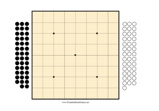
If you use same deterministic strategy, your network will always place the stone in a “particular” position which is a highly undesirable behaviour since it makes you predictable by your opponent. In that situation, a stochastic policy is more suitable than deterministic policy.
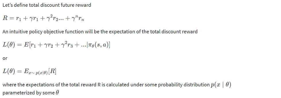
Policy Objective Functions :
So how can I find πθ(s,a)? Actually, we can use the reinforcement technique to solve it. For example, suppose the drone is trying to reach our specified location. At the beginning the drone may simply not reach the target location and may go out of the bound and receive a negative reward, so the neural network will adjust the model parameters θ such that next time it will try to avoid going out of the bound. After many attempts it will have discovered that “argh if I dont overcross the range specified I may reach the destination”. In mathematics language, we call these policy objective functions.
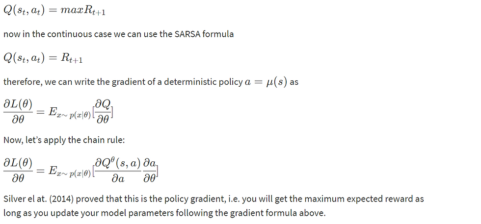
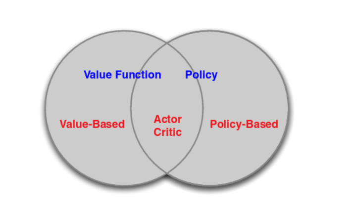
Actor-Critic Algorithm :
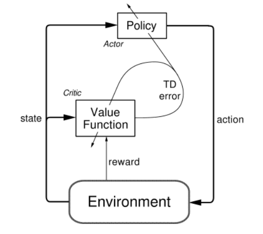
The Actor-Critic Algorithm is essentially a hybrid method to combine the policy gradient method and the value function method together. The policy function is known as the actor, while the value function is referred to as the critic. Essentially, the actor produces the action a given the current state of the environment s, while the critic produces a signal to criticizes the actions made by the actor. I think it is quite natural in the human’s world where the junior employee (actor) do the actual work and your boss (critic) criticizes your work and hopefully the junior employee can do it better next time. In our project, we use the continuous Q-learning (SARSA) as our critic model and use policy gradient method as our actor model. The following figure explains the relationships between Value Function/Policy Function and Actor-Critic Algorithm.
We need to make 2 files
1) Drone_Task.PY : We will define our task (environment) in this file.
2) Drone_Agent.PY : To develop our reinforcement learning agents
The Task for drone :
The code and explanation is given below .The attempted task for our drone is to take-off vertically and then hover at height 30. I provided the agent with the 6D target pose. The reward function was designed to encourage the drone to vertically take off and stay within range of the target position in the vertical axis. I then clipped the reward to have within [-1,1] range to facilitate learning through the Neural Networks and avoid exploding gradients.
reward = -.03(abs(self.sim.pose[2] - self.target_pos[2])) + .005self.sim.v[2] reward = np.clip(reward, -1, 1)
import numpy as np
from physics_sim import PhysicsSim

class TakeOff():
    """Task (environment) that defines the goal and provides feedback
       to the agent."""
    def __init__(self, init_pose=None, init_velocities=None,
        init_angle_velocities=None, runtime=5., target_pos=None):
        """Initialize a Task object.
        Params
        ======
            init_pose: initial position of the quadcopter in (x,y,z)
            dimensions and the Euler angles
            init_velocities: initial velocity of the quadcopter in
            (x,y,z) dimensions
            init_angle_velocities: initial radians/second for each of
            the three Euler angles
            runtime: time limit for each episode
            target_pos: target/goal (x,y,z) position for the agent
        """
        # Simulation
        self.sim = PhysicsSim(init_pose, init_velocities,
        init_angle_velocities, runtime)
        self.action_repeat = 3

        self.state_size = self.action_repeat * 6
        self.action_low = 0
        self.action_high = 900
        self.action_size = 4

        # Goal
        self.target_pos = target_pos if target_pos is not None else
           np.array([0., 0., 10.])

    def get_reward(self):
        reward=-.03*(abs(self.sim.pose[2] -self.target_pos[2]))             +.005*self.sim.v[2]
        reward=np.clip(reward, -1, 1)
        return reward

    def step(self, rotor_speeds):
        """Uses action to obtain next state, reward, done."""
        reward = 0
        pose_all = []
        for _ in range(self.action_repeat):
            done = self.sim.next_timestep(rotor_speeds) # update the
            sim pose and velocities
            reward += self.get_reward()
            pose_all.append(self.sim.pose)
        next_state = np.concatenate(pose_all)
        return next_state, reward, done

    def reset(self):
        """Reset the sim to start a new episode."""
        self.sim.reset()
        state = np.concatenate([self.sim.pose] * self.action_repeat)
        return state
The __init__() method is used to initialize several variables that are needed to specify the task.
The simulator is initialized as an instance of the PhysicsSim class (from physics_sim.py).
Inspired by the methodology in the original DDPG paper, we make use of action repeats. For each timestep of the agent, we step the simulation action_repeats timesteps. If you are not familiar with action repeats, please read the Results section in the DDPG paper.
We set the number of elements in the state vector. For the sample task, we only work with the 6-dimensional pose information. To set the size of the state (state_size), we must take action repeats into account.
The environment will always have a 4-dimensional action space, with one entry for each rotor (action_size=4). You can set the minimum (action_low) and maximum (action_high) values of each entry here.
The sample task in this provided file is for the agent to reach a target position. We specify that target position as a variable.
The reset() method resets the simulator. The agent should call this method every time the episode ends. You can see an example of this in the code cell below.
The step() method is perhaps the most important. It accepts the agent's choice of action rotor_speeds, which is used to prepare the next state to pass on to the agent. Then, the reward is computed from get_reward(). The episode is considered done if the time limit has been exceeded, or the quadcopter has travelled outside of the bounds of the simulation.
Keras Code Explanation :
Our agent will consist of following functions .
1)Replay Buffer
2)Actor Network
3)Critic Network
4)DDPG Agent
5)OU Noice
File : Drone_agent.py
Lets understand each function
Replay Buffer :
Most modern reinforcement learning algorithms benefit from using a replay memory or buffer to store and recall experience tuples.
Here is a sample implementation of a replay buffer that you can use:
import random
from collections import namedtuple, deque

class ReplayBuffer:
    """Fixed-size buffer to store experience tuples."""

    def __init__(self, buffer_size, batch_size):
        """Initialize a ReplayBuffer object.
        Params
        ======
            buffer_size: maximum size of buffer
            batch_size: size of each training batch
        """
        self.memory = deque(maxlen=buffer_size)  # internal memory (deque)
        self.batch_size = batch_size
        self.experience = namedtuple("Experience", field_names=
        ["state", "action", "reward", "next_state", "done"])

    def add(self, state, action, reward, next_state, done):
        """Add a new experience to memory."""
        e = self.experience(state, action, reward, next_state, done)
        self.memory.append(e)

    def sample(self, batch_size=64):
        """Randomly sample a batch of experiences from memory."""
        return random.sample(self.memory, k=self.batch_size)

    def __len__(self):
        """Return the current size of internal memory."""
        return len(self.memory)
Actor(policy) Network:
Let’s first talk about how to build the Actor Network in Keras. Here we used 3 hidden layers with 32 , 64 and 32 hidden units respectively with relu activation function. The output consist of 4 continuous actions(Rotor Speeds) with sigmoid activation function.
from keras import layers, models, optimizers
from keras import backend as K

class Actor:
    """Actor (Policy) Model."""

    def __init__(self, state_size, action_size, action_low,
         action_high):
         Params
        ======
            state_size (int): Dimension of each state
            action_size (int): Dimension of each action
            action_low (array): Min value of each action dimension
            action_high (array): Max value of each action dimension
        """
        self.state_size = state_size
        self.action_size = action_size
        self.action_low = action_low
        self.action_high = action_high
        self.action_range = self.action_high - self.action_low
        self.build_model()

    def build_model(self):
        """Build an actor (policy) network that maps states ->
         actions."""
        # Define input layer (states)
        states = layers.Input(shape=(self.state_size,), name='states')

        # Add hidden layers
        net = layers.Dense(units=32, activation='relu')(states)
        net = layers.Dense(units=64, activation='relu')(net)
        net = layers.Dense(units=32, activation='relu')(net)

        # Try different layer sizes, activations, add batch
         normalization, regularizers, etc.

        # Add final output layer with sigmoid activation
        raw_actions = layers.Dense(units=self.action_size,
           activation='sigmoid' , name='raw_actions')(net)

        # Scale [0, 1] output for each action dimension to proper range
        actions = layers.Lambda(lambda x: (x * self.action_range) +
           self.action_low, name='actions')(raw_actions)

        # Create Keras model
        self.model = models.Model(inputs=states, outputs=actions)

        # Define loss function using action value (Q value) gradients
        action_gradients = layers.Input(shape=(self.action_size,))
        loss = K.mean(-action_gradients * actions)

        # Incorporate any additional losses here (e.g. from
           regularizers)

        # Define optimizer and training function
        optimizer = optimizers.Adam()
        updates_op =
        optimizer.get_updates(params=self.model.trainable_weights,
         loss=loss)
        self.train_fn = K.function(
            inputs=[self.model.input, action_gradients,
            K.learning_phase()],
            outputs=[],
            updates=updates_op)
Note that the raw actions produced by the output layer are in a [0.0, 1.0] range (using a sigmoid activation function). So, we add another layer that scales each output to the desired range for each action dimension. This produces a deterministic action for any given state vector. A noise will be added later to this action to produce some exploratory behavior.
Another thing to note is how the loss function is defined using action value (Q value) gradients
These gradients will need to be computed using the critic model, and fed in while training. Hence it is specified as part of the "inputs" used in the training function
Critic(Value) Model:
The construction of the Critic Network is very similar to the Deep-Q Network. The critic network takes both the states and the action as inputs. According to the DDPG paper, the actions were not included until the 2nd hidden layer of Q-network. Here we used the Keras function Merge to merge the action and the hidden layer together .
class Critic:
    """Critic (Value) Model."""

    def __init__(self, state_size, action_size):
        Params
        ======
            state_size (int): Dimension of each state
            action_size (int): Dimension of each action
        """
        self.state_size = state_size
        self.action_size = action_size

        self.build_model()

    def build_model(self):
        """Build a critic (value) network that maps (state, action)
         pairs -> Q-values."""
        # Define input layers
        states = layers.Input(shape=(self.state_size,), name='states')
        actions = layers.Input(shape=(self.action_size,),
        name='actions')

        # Add hidden layer(s) for state pathway
        net_states = layers.Dense(units=32, activation='relu')(states)
        net_states = layers.Dense(units=64, activation='relu')(net_states)

        # Add hidden layer(s) for action pathway
        net_actions = layers.Dense(units=32, activation='relu')(actions)
        net_actions = layers.Dense(units=64, activation='relu')(net_actions)

        # Try different layer sizes, activations, add batch
        normalization, regularizers, etc.

        # Combine state and action pathways
        net = layers.Add()([net_states, net_actions])
        net = layers.Activation('relu')(net)

        # Add more layers to the combined network if needed

        # Add final output layer to prduce action values (Q values)
        Q_values = layers.Dense(units=1, name='q_values')(net)

        # Create Keras model
        self.model = models.Model(inputs=[states, actions],
        outputs=Q_values)

        # Define optimizer and compile model for training with built-in
        loss function
        optimizer = optimizers.Adam()
        self.model.compile(optimizer=optimizer, loss='mse')

        # Compute action gradients (derivative of Q values w.r.t. to
        actions)
        action_gradients = K.gradients(Q_values, actions)

        # Define an additional function to fetch action gradients (to
        be used by actor model)
        self.get_action_gradients = K.function(
            inputs=[*self.model.input, K.learning_phase()],
            outputs=action_gradients)
It is simpler than the actor model in some ways, but there some things worth noting. Firstly, while the actor model is meant to map states to actions, the critic model needs to map (state, action) pairs to their Q-values. This is reflected in the input layers.
These two layers can first be processed via separate "pathways" (mini sub-networks), but eventually need to be combined. This can be achieved, for instance, using the Add layer type in Keras (see Merge Layers)
The final output of this model is the Q-value for any given (state, action) pair. However, we also need to compute the gradient of this Q-value with respect to the corresponding action vector, needed for training the actor model. This step needs to be performed explicitly, and a separate function needs to be defined to provide access to these gradients
DDPG Agent:
We are now ready to put together the actor and policy models to build our DDPG agent. Note that we will need two copies of each model - one local and one target. This is an extension of the "Fixed Q Targets" technique from Deep Q-Learning, and is used to decouple the parameters being updated from the ones that are producing target values.
Here is an outline of the agent class:
class DDPG():
    """Reinforcement Learning agent that learns using DDPG."""
    def __init__(self, task):
        self.task = task
        self.state_size = task.state_size
        self.action_size = task.action_size
        self.action_low = task.action_low
        self.action_high = task.action_high

        # Actor (Policy) Model
        self.actor_local = Actor(self.state_size, self.action_size,
        self.action_low, self.action_high)
        self.actor_target = Actor(self.state_size, self.action_size,
        self.action_low, self.action_high)

        # Critic (Value) Model
        self.critic_local = Critic(self.state_size, self.action_size)
        self.critic_target = Critic(self.state_size, self.action_size)

        # Initialize target model parameters with local model
        parameters
        self.critic_target.model.set_weights(self.critic_local.model.get_weights())
        self.actor_target.model.set_weights(self.actor_local.model.get_weights())

        # Noise process
        self.exploration_mu = 0
        self.exploration_theta = 0.15
        self.exploration_sigma = 0.2
        self.noise = OUNoise(self.action_size, self.exploration_mu, self.exploration_theta, self.exploration_sigma)

        # Replay memory
        self.buffer_size = 100000
        self.batch_size = 64
        self.memory = ReplayBuffer(self.buffer_size, self.batch_size)

        # Algorithm parameters
        self.gamma = 0.99  # discount factor
        self.tau = 0.01  # for soft update of target parameters

    def reset_episode(self):
        self.noise.reset()
        state = self.task.reset()
        self.last_state = state
        return state

    def step(self, action, reward, next_state, done):
         # Save experience / reward
        self.memory.add(self.last_state, action, reward, next_state, done)

        # Learn, if enough samples are available in memory
        if len(self.memory) > self.batch_size:
            experiences = self.memory.sample()
            self.learn(experiences)

        # Roll over last state and action
        self.last_state = next_state

    def act(self, state):
        """Returns actions for given state(s) as per current policy."""
        state = np.reshape(state, [-1, self.state_size])
        action = self.actor_local.model.predict(state)[0]
        return list(action + self.noise.sample())  # add some noise for exploration

    def learn(self, experiences):
        """Update policy and value parameters using given batch of experience tuples."""
        # Convert experience tuples to separate arrays for each element (states, actions, rewards, etc.)
        states = np.vstack([e.state for e in experiences if e is not None])
        actions = np.array([e.action for e in experiences if e is not None]).astype(np.float32).reshape(-1, self.action_size)
        rewards = np.array([e.reward for e in experiences if e is not None]).astype(np.float32).reshape(-1, 1)
        dones = np.array([e.done for e in experiences if e is not None]).astype(np.uint8).reshape(-1, 1)
        next_states = np.vstack([e.next_state for e in experiences if e is not None])

        # Get predicted next-state actions and Q values from target models
        #     Q_targets_next = critic_target(next_state, actor_target(next_state))
        actions_next = self.actor_target.model.predict_on_batch(next_states)
        Q_targets_next = self.critic_target.model.predict_on_batch([next_states, actions_next])

        # Compute Q targets for current states and train critic model (local)
        Q_targets = rewards + self.gamma * Q_targets_next * (1 - dones)
        self.critic_local.model.train_on_batch(x=[states, actions], y=Q_targets)

        # Train actor model (local)
        action_gradients = np.reshape(self.critic_local.get_action_gradients([states, actions, 0]), (-1, self.action_size))
        self.actor_local.train_fn([states, action_gradients, 1])  #
        custom training function

        # Soft-update target models
        self.soft_update(self.critic_local.model,
        self.critic_target.model)
        self.soft_update(self.actor_local.model,
        self.actor_target.model)

    def soft_update(self, local_model, target_model):
        """Soft update model parameters."""
        local_weights = np.array(local_model.get_weights())
        target_weights = np.array(target_model.get_weights())

        assert len(local_weights) == len(target_weights), "Local and
        target model parameters must have the same size"

        new_weights = self.tau * local_weights + (1 - self.tau) *
        target_weights
        target_model.set_weights(new_weights)
Notice that after training over a batch of experiences, we could just copy our newly learned weights (from the local model) to the target model. However, individual batches can introduce a lot of variance into the process, so it's better to perform a soft update, controlled by the parameter tau.
One last piece you need for all this to work properly is an appropriate noise model, which is presented next.
Ornstein–Uhlenbeck Noise :
What is Ornstein-Uhlenbeck process? In simple English it is simply a stochastic process which has mean-reverting properties.
dxt=θ(μ−xt)dt+σdWt
here, θ means the how “fast” the variable reverts towards to the mean. μ represents the equilibrium or mean value. σ is the degree of volatility of the process.
import numpy as np
import copy

class OUNoise:
    """Ornstein-Uhlenbeck process."""

    def __init__(self, size, mu, theta, sigma):
        """Initialize parameters and noise process."""
        self.mu = mu * np.ones(size)
        self.theta = theta
        self.sigma = sigma
        self.reset()

    def reset(self):
        """Reset the internal state (= noise) to mean (mu)."""
        self.state = copy.copy(self.mu)

    def sample(self):
        """Update internal state and return it as a noise sample."""
        x = self.state
        dx = self.theta * (self.mu - x) + self.sigma *
        np.random.randn(len(x))
        self.state = x + dx
        return self.state
Training :

The actual training of the neural network is very simple, only contains few lines of code:
from task import Task
from agents.agent import DDPG
## The task I chose to focus on is to perform a TAKE-OFF operation to height 20
from task import TakeOff

# Quadcopter starting position parameters
runtime = 5.                                     # time limit
init_pose = np.array([0., 0., 10., 0., 0., 0.])   # initial pose
init_velocities = np.array([0., 0., 0.])         # initial velocities
init_angle_velocities = np.array([0., 0., 0.])   # initial angle velocities
done = False # initialise done bool variable

num_episodes = 1000 # simulation will run for 500 episodes
target_pos = np.array([0., 0., 30., 0., 0., 0.])             # target height is 20

# select task of interest
task = TakeOff(init_pose = init_pose,
               init_velocities = init_velocities,
               init_angle_velocities = init_angle_velocities,
               target_pos = target_pos,
               runtime = runtime)
# select agent to perform the task of interest
agent = DDPG(task)

file_output1 = 'TakeOff-data.txt' # file name for saved results

labels = ['time', 'x', 'y', 'z', 'phi', 'theta', 'psi', 'x_velocity',
 'y_velocity', 'z_velocity', 'phi_velocity', 'theta_velocity',
 'psi_velocity', 'rotor_speed1', 'rotor_speed2', 'rotor_speed3', 'rotor_speed4',
 'episode', 'total_reward']
results = {x : [] for x in labels}

# Run the simulation, and save the results.
# In this while loop, we get both a summary text output from this cell,
# and results saved in a txt file
with open(file_output, 'w') as csvfile:
    writer = csv.writer(csvfile)
    writer.writerow(labels)

 for i_episode in range(1, num_episodes+1):
        state = agent.reset_episode() # start a new episode
 while True:
            action = agent.act(state)
            next_state, reward, done = task.step(action)
            agent.step(action, reward, next_state, done)
            state = next_state
 if done:
 # get summary text output
 print("\r Total Number of Episode = {:4d}, Total Score = {:7.3f}, Best Recorded Score = {:7.3f}".format(
                    i_episode, agent.total_reward, agent.best_total_reward), end="")  # [debug]
 # and save results in text file
                to_write = [task.sim.time] + list(task.sim.pose) + list(task.sim.v) + list(task.sim.angular_v) + list(action) + [i_episode] + [agent.total_reward]
 for ii in range(len(labels)):
                    results[labels[ii]].append(to_write[ii])
                writer.writerow(to_write)
 #print(task.sim.pose[:3])
 break
        sys.stdout.flush()
Validation and Performance :
As we develop the agent, it's important to keep an eye on how it's performing. Use the code above as inspiration to build in a mechanism to log/save the total rewards obtained in each episode to file. If the episode rewards are gradually increasing, this is an indication that your agent is learning.
plt.plot(results['episode'], results['total_reward'])
_ = plt.ylim()
plt.title("Score over 1000 episodes");
rolling_mean = pd.Series(results['total_reward']).rolling(50).mean()
plt.plot(rolling_mean);
Here's what I got !
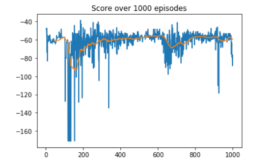
The agent did a decent work at learning to take off vertically and hover to a target location within range. The best score achieved was -1.78 with the average over the last 10 episodes at -72.6 and the worst recorded score at -171.1. There was no particular 'aha' moment but it is clear that the agent was trying to different approaches before settling on a policy in the last dozen episodes which indicates that the agent did in fact go through a learning curve.
Summary:
Congratulations , you made it till here ! In this project, we managed to teach quadcopter how to fly using Keras and DDPG algorithm . Although the DDPG can learn a reasonable policy, I still think it is quite different from how humans learn to drive. For example, we used Ornstein-Uhlenbeck process to perform the exploration. However, when the number of actions increase, the number of combinations increase and it is very challenging to do the exploration.
However, having said that the algorithm is quite powerful because we have a model-free algorithm for continuous control, which is very important in robotics.
In my next blog I will show the simulation video output of the Drone.
Here's a joke for you after some heedful and complicated stuff : If you are somehow able to set Drone's speed to 11.2 km/sec , it can even reach the space :)
Comments